The use of “Formula”
We use “Formula” to calculate values, or apply mathematical “Function”(s) to “Cells”.
There are two ways to write these “Formula”(s)
By means of a “Range Syntax”, or the “Simple Syntax”.
“Syntax” means the manner in which the “Formula”(s) will be written.
We can do both for more complex “Formula”(s).
We use the “Simple Syntax” for different calculations in different”Cells”.
We use the “Range Syntax” if we only want to perform a calculation on a “Range” of “Cells”.
We can always change a “Formula” later.
To do this select the cell containing the “Formula” in the “Formula” bar and you can make changes.
“Simple Syntax” formulas
For a “Formulas”,we first select the cell where we wish to have the result.
Then we type an ‘=’ sign in the “Formula” bar. A “Formula” always begins with an ‘=’ sign.
And then we type our “Formula”.
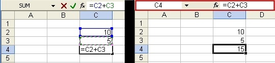
When we click “Enter”, it gives us the result in our Excel “Spreadsheet”.
Note that the contents of cell C4 is still our “Formula”.
Excel displays the “Formula” as text anyway, so you should first see if you typed space before the ‘=’ sign. A “Formula” must begin with the ‘=’ sign.
Though, the actual content of the cell is the “Formula”, the cell displays the result.eg: =
A1 + A2 + A3 + A4
Exactly the same as what we have learned in school.
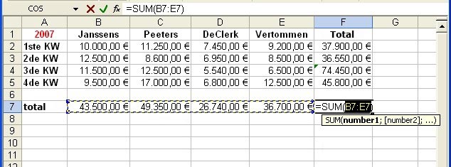
“Range Syntax” formulas
If we want to enter “Range Syntax” formulas, we start as in the “Simple Syntax” “Formula”, first select the cell where we want the result to be displayed and then we type an ‘=’ sign in the “Formula” bar.
Then we type the function, followed by an open parenthesis “(” , followed by the range, and finally we close the parenthesis “)”, and click “Enter”.
We do not use spaces in our formulas.
eg:= SUM (A1: A4)
I’ll start with the = sign, then the function and then the “Range” in brackets
If we use both syntaxes in a “Formula”, this would be like: = SUM (C2: C3) * 21%
In the first part we use a function and in the second part, a calculation
“Formula”(s) that refer to a cell will be instantly updated when the content of this cell is changed. This means we need not always update the formulas.
This is one of the best features of Excel, and one of the reasons we have minimal entry of the numbers in “Formula”(s).
When we insert cell addresses in a “Formula” we can simply type them, or just click the mouse in the cell, select and drag the selected range of cells that we want to enter.
If the “Formula” is typed, we click the “Enter” key, and see the results immediately.
Arithmetic operations:
| Add | + | Multiply | * |
| Subtract | – | Percentage | % |
| Divide | / | Exponentiation | ^ |
Excel uses a specific order in the calculations.
If you want to record multiple operations in a “Formula”, it is somewhat more difficult.
Excel will calculate the percentage first, then perform the exponentiation, then multiply or divide are carried out at the same level to be treated from left to right and finally addition and subtraction are also carried out, at the same level from left to right eg:
| 1.Percentage | % | |||
| 2.Exponentiation | ^ | |||
| 3.multiply and divide | * and / | |||
| 4.add and subtract | + and – |
“Formula” functions
In a “Range Syntax” formula we can only give a single function to one or more area (s) of cells.
There are many functions that we can use such as Sine and Cosine and other complicated functions, but unless we are in a specialized field as an accountant or an engineer, we will almost never use it.
The most obvious features that we are going to use are as follows:
“Sum” (“Sum”), “Average” (“Average“), “Max” (“Max”), “Min” (“Min”) and “Count” (“Count”).
The use of “AutoSum”
Very often we use Excel to calculate totals of columns or rows.
So often that they have even added a “AutoSum” ![]() in Excel.
in Excel.
This button automatically calculates the totals of rows or columns.
For this purpose we choose an empty cell, at the end of a column or row.
We click the “AutoSum” button.
Excel gives us a proposal of what “Range” it wants to calculate the total.
If the proposed range is not correct, click and drag over the cells you want to see in your “Range”.
Finally we click the “AutoSum” button again or we click the “Enter” button.
A second way to do this is, click on an empty cell, select all the cells in your “Range” and click the “AutoSum” button.
Excel gives you the total amount of all these cells in the empty cell.
In Office XP and 2003, the “AutoSum” button is not limited only to calculate the sum.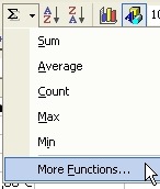
When you click on the black arrow on the right side, you have more choice of modes in a dropdown menu.
If the function you are looking for is not listed, click on the selection “More Functions…” (“More Functions …”)
More on this in the next section of this lesson.
Entering “Functions” (XP and 2003)
In Excel XP and 2003, we can enter “Functions” in three ways:
- In the menu bar click on “Insert” – “Function “
- Click on the”fx” button in the “Formula” bar
- Or select “More Functions …” from the dropdown list that you see when you click on the black arrow next to the “AutoSum”.
When one of these actions happens, you get an “Insert Function” dialog box:
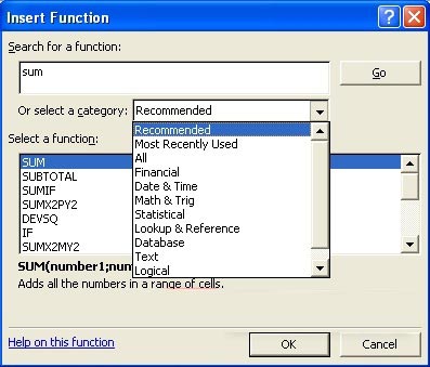
In the “Insert Function” dialog box we can find a function by typing a few words in the “Search for a function:” text box and clicking “Ok.”
A list will appear with designated “Functions” from which we can make a choice.
Click on a feature to see a description and “Syntax” (spelling) of this “Function”.
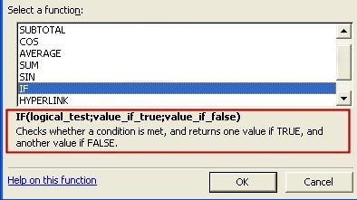
Or we can choose a “Function” from the dropdown list by clicking on the arrow next to “Select a category:”
If you choose the “All” category, you’ll see an alphabetical list of all “Functions” in Excel.
Again, we can select a “Function” and see its “Syntax” and descriptions.
Once a “Function” is selected, click the OK button at the bottom.
This gives us the “Function Arguments” dialog box.
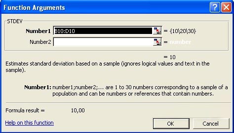
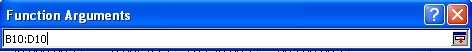
Here we click the Collapse/Expand Dialog Box button ![]() to close the dialog box to make it easier for us to select a “Range” in our “Worksheet”.
to close the dialog box to make it easier for us to select a “Range” in our “Worksheet”.
Then we select the “Range” where we want to apply the “Function”.
We again click the Collapse/Expand Dialog Box button ![]() , and click OK in the “Function Arguments” dialogbox, to add the “Function” in our “Worksheet”.
, and click OK in the “Function Arguments” dialogbox, to add the “Function” in our “Worksheet”.
Editing a “Range” (XP and 2003)
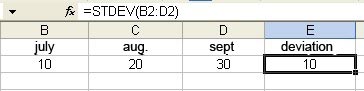
We can still change the “Range” in a “Formula” after we entered it.
To do this we double-click the cell containing the “Formula”.
This gives the appearance to our cell as a “Formula”, instead of the value, and indicates the “Range” in a blue frame.
We bring our pointer now to one of the corners of the framework, we can increase or decrease to our “Range”.
We bring our mouse pointer over a line of our framework and can drag the whole range to another place.
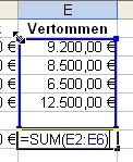
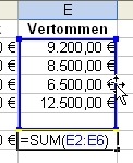
When either occurs, the “Formula” will automatically adjust.
” AutoCorrect” “Formula”
When you enter a “Formula”, Excel will try to assist you in writing the correct “Syntax”. When you insert spaces or additional processing, Excel will display a dialog box in which it proposes the correct “Syntax”:
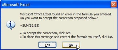
Click “Yes” to accept the proposal, click “No” to correct the error by yourself.
“AutoCalculate” (“AutoCalculate”)
“AutoCalculate” is a temporary expedient that displays the results of simple calculations in the Status bar without having to type a “Formula”.
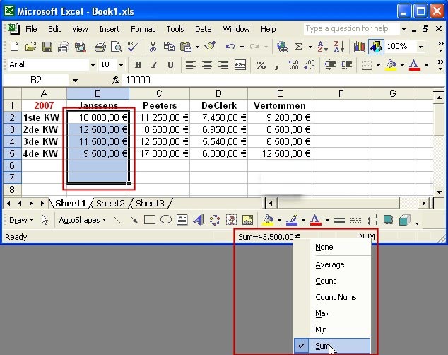
Select the “Range” in our “Worksheet”.
Now right click the mouse button on the “Status bar”. We see a combo box where we can make our choice.
We can choose from “None”, “Average”, “Count”, “Count Nums”, “Max”, “Min” and “Sum “.
Whatever choice you make, the result will be shown in the “Status bar” as long as our “Range” remains selected.


