What is a “Function”?
“Functions” ensure that certain calculations are carried out in a fast way.
Examples of “Functions” eg = SUM (), = AVERAGE (), etc. ..
“Search functions” (“Search function”)
There are two “Functions” that we use to retrieve data.
The first “HLOOKUP” (“HLOOKUP”), looks for a value in a table that is structured in rows (with column headings on the right side)
The second and more common is the “VLOOKUP” (“VLOOKUP”), can locate a value in a traditional column table.
Based on the design of the table where we want to search, we have to enter one of the two “Search functions” mentioned above.
“Search functions” have several arguments to work with.
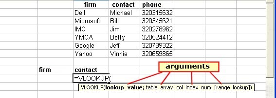
The first three must be completed but, the fourth is optional, and has a logic value: (“TRUE” or “false”)
The first argument is the “Lookup_value”: this is the value we want to find in our table. This can either be a value that we type or a cell reference.
The second argument is the “Table_array”: it is the “Range” of cells in our table where we want to find our first argument.
The third argument is “Col_index_num”: here we give the column number or row number, where we have the information.

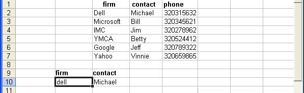
If we just analyze the picture above we see that the first argument is B10, this will be the cell where we enter the value which we want to find information.
For the second argument I give the range, where it must look as C1: E7.
And in the third argument I give the column number where the information can be found, in our case it is 2 (2nd column from our range)
If we want search for an exact match, we can enter FALSE as the fourth argument.
If we want to copy the “Formula”, we need to make the second argument, our “Range”,an “Absolute cell reference”: $ C $ 1: $ E $ 7.
But that should be clear, if you have gone through all the previous lessons.
“Logical Functions”
“Logical functions” are useful in order to display different results in a cell, based on the contents of another cell.
Logical functions are:
| Dutch | English | Explanation |
| AND | AND | Returns the result TRUE if all arguments are TRUE |
| FALSE | FALSE | Returns the logical value- FALSE. |
| AS | IF | Indicates a value when the condition is TRUE and another value if FALSE. |
| NOT | NOT | We use NOT to check if a value is not equal to another value. |
| OR | OR | Returns TRUE if at least one of the arguments is TRUE. |
| WHERE | TRUE | Returns the logical value TRUE. |
For a Boolean function, we have to write at least three arguments.
1. The test which assesses the cell value.
2. The cell value when the test is successful.
3. The cell value if the test fails..
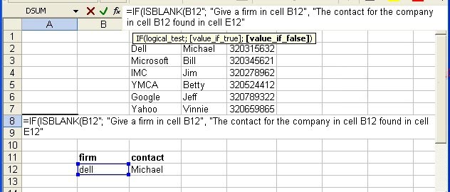
Below I have made an example.
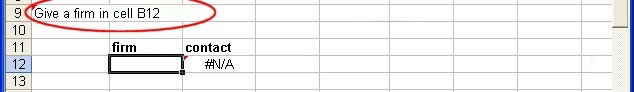
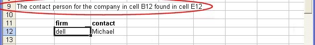
If no firm is entered in cell B12, it displays the text “Give a firm, in cell B12” in cell A9
When a firm is found it gives the text “The contact for the company in cell B12 found in cell E12” .
These are the arguments that we need:
The first argument = IF (ISBLANK (B12)
The second argument: “Give a firm, in cell B12”
The third argument: “The contact for the company in cell B12 found in cell E12”)
Between two arguments we place a ‘;’ (semi colon) sign
Result FALSE
Result TRUE
Another example would be:
If a seller has a certain turnover, he gets a bonus on his wages.
It is this formula: = IF (C50> C48, SUM (C50* D48) 😉
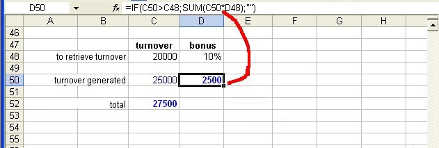
This “Formula” is made with cell references, so we can easily change all amounts and percentages without having to adjust our “Formula”.
The nesting of “Logical functions”
A “nested logical function” is a feature that prevents multiple IF statements.
We can use up to 7 IF statements in a “Formula”.
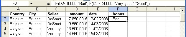
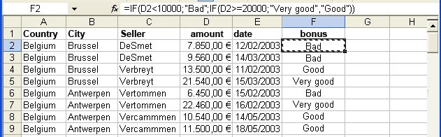
An example: = IF (D2 <10000; “Bad”, IF (D2> = 20000; “Very good”, “Good”))
So if the cell D2 (the amount) is less than 10,000 it gives us the message “Bad”.
If the cell D2 is greater than or equal to 20,000, it gives us is the statement “Very good”.
If it is neither of the two, it gives us the message “Good”.
Keep in mind that every IF statement must conclude with a ‘)’ at the end of the “Formula”.
We can copy the “Formula” to other cells.
Suppressing “Error messages”
In complicated spreadsheets, it can happen that we get an error because no values are entered in certain cells.
A good example is the “VLOOKUP” (VLOOKUP).
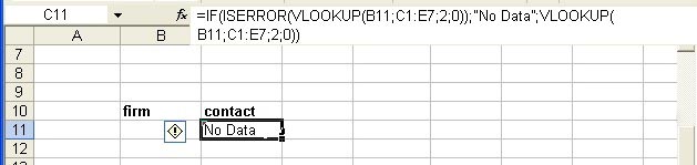
When we have no firm entered we get to see this: ‘# N / A ”
We can use the “ISERROR” (“ISERROR”) “Function”, in cooperation with the “IF” (“IF”) “Function” to show an “Error Message” when our “Formula” encounters an error.
The syntax for this is:
= IF (ISERROR (VLOOKUP (B11; C1: E7; 2, 0)); “No Data”; VLOOKUP (B11; C1: E7; 2; 0))
This is explained as
= IF (ISERROR (“Function” being tested); “Error message”; (and the function when there is no error)).
In Excel XP and 2003 we can hide the “Error messages” when printing “Formulas”.
This is something we have seen in a previous lesson.
But remember:
Choose “File” in the menu bar, select “Page Setup”.
In the dialog, we select the tab “Sheet”
And the drop-down menu of “Cell errors as:” we make our choice.
The use of “AND” and “OR” functions
If we want to check if a cell meets certain conditions, we use the “AND” and “OR” “Functions”.
The “AND” “Function” returns a TRUE value when both conditions are met.
The “OR” “Function” gives a TRUE value when one of the conditions is satisfied.
We take an example of our sales representatives.
We want to calculate a bonus based on the turnover, taking into account the region in which they sell and only when we are paid by our customers.
In the first worksheet have our sales list:
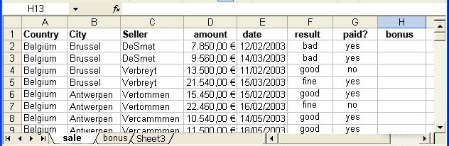
Here we find the field ‘City”, “Country”, “Salesperson”, “amount”, ‘date”, “result”, and “bonus pay”.
The field in which a “Formula” is entered is the “result” column , which relies on the cell “amount” with the following “Formula”: = IF (D2 <10000; “bad”, IF (D2> = 20000; “fine”; “good”))
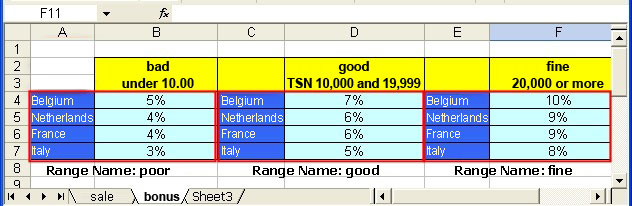
In the second “Worksheet” in our “Workbook”, we have different bonuses for different regions:
We have created three “Ranges” in this “Worksheet”: low (A4: B7), good (C4: D7) and fine (E4: F7)
(Lesson 12 shows you how to give a name to a “Range”)
So what we want to know is, the region in which the seller is located, which bonus is applied to this order and whether our customer has paid or not.
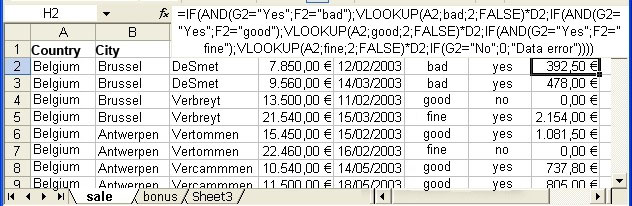
We type so the “Formula” in cell H2 of the sales “Worksheet”:
= IF (AND (G2 = “Yes”, F2 = “bad”); VLOOKUP (A2, bad, 2, FALSE)* D2; IF (AND (G2 = “Yes”, F2 = “good”) IF ( AND(G2 = “Yes”, F2 = “fine”);VLOOKUP (A2, fine, 2, FALSE) *D2; IF (G2 = “No”, 0, “Data error”))))
I will try to explain the “Formula”: (Emphasis is on try)
= IF (AND (G2 = “Yes”, F2 = “bad”); VLOOKUP (A2, bad, 2, FALSE) *D2;)
As always we start the “Formula” with an = sign, then we type IF (IF)
Then we use the AND (S) function because we have to meet several conditions.
The first condition is that the cell G2 should be equal to Yes, if it is not paid, we have no bonus.
And if the second condition is “bad”.
We then search the region A2 in the worksheet in the bonus area “(bad)” in the 2nd column (2), with an exact equation (FALSE).
Then we multiply this value with the cell D2
IF (AND (G2 = “Yes”, F2 = “good”), VLOOKUP (A2, good, 2, FALSE) * D2;
Then we type this again, but now for the cell “result” and the “Range” name “good”
IF (AND (G2 = “Yes”, F2 = “fine”), VLOOKUP (A2, fine, 2, FALSE)* D2;
And again, but now for the cell “result” and the range name “fine”
IF (G2 = “No”, 0, “Data error”))))
What we finally want to check if the cell for paid is “No”, if so it must give the value as 0, if not, perhaps because someone forgot to fill it in by mistake, then it should display the “data error” message.
We do not forget to conclude the end of our IF “Formula” conditions with a ‘)’ sign
We have therefore four))))
Once this “Formula” works, we can copy them to the fields below.


