Creating a new “Workbook” (“Workbook”)
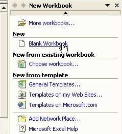
To create a new “Workbook”, we click the ‘File” menu and select “New” (“New File”) Or simply click on the “Blank Workbook” on the “Task Panel”.
When you use Excel XP or 2003, select “File” – “New” (“Blank Workbook”). In the “Task Panel”, you choose “Blank Workbook”.
When you use Excel ’97 or 2000, select “File” – “New”, a dialog box will appear where you select “Workbook” from the “General” tab.
Click on OK.
“Workbook”
After inserting data into our new “Worksheet” we should store the information so that it is not lost.
We click on the “Save” button. (“Save”) 
Select a folder where you want to save the file, give it a name, and click OK.
Remember where you saved the file and be sure what you’ve named the file.
This can save a lot of time when you want to “Edit” the file later.
Closing files
To close the file we click the “File” and select “Close” (“File – Close”),
We can also click the X in the upper right corner of our “Workbook”.
Warning! Do not click the X in the upper right corner of the application, because then you close the “Excel” program.
“Excel” will ask if you want to save the file, click YES if you wish to or else click NO.
Opening files
If you want to open a file, the first thing you should know is where this file is located.
Is it somewhere in a folder on your hard drive, is it on a CD-ROM or floppy disk?
Once you know where the file is located, click the “Open” button.
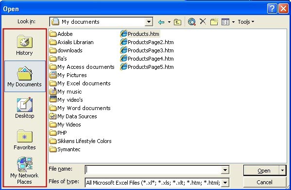
A dialog box appears, locate the file, select it and click “Open”.
If you want to open multiple files, hold the “Shift” button on your keyboard, select all files and click “Open”
In the version of Excel 2000, XP and 2003, we have shortcuts to frequently used folders on the left of the dialog box .
Selecting “Cells”
When we open a new “Workbook”, the selected “Cell” is always A1.
You can use your mouse to click in any “Cell” to make it “active”.
We can use the arrow keys on our keyboard to scroll through the “Cells”.
There are many different ways to select “Cells”, below is a list:
| “UP” arrow key | moves the active cell upward |
| “DOWN” arrow key | moves the active cell downward |
| “LEFT” arrow key | moves the active cell to the left |
| “RIGHT” arrow key | moves the active cell to the right |
| “Pg Up” key | moves the active cell up by one page |
| “Pg Dn” key | moves the active cell down by one page |
| “Alt”+ “Pg Up” key | moves the active cell one page to the left |
| “Alt” + “Pg Dn” key | moves the active cell one page to the right |
| “Ctrl”+”Home” key | moves the active cell to the left-most cell |
| “Ctrl”+”End” key | moves the active cell to the lowest right cell |
| “Tab” key | moves the active cell one cell to the right |
| “Shift”+ “Tab” key | moves the active cell one cell to the left |
| “Enter” key | moves to the active cell to a subject |
| “Shift”+ “Enter” key | moves the active cell one cell upward |
Insert text in cells
In “Excel”, a combination of numbers and text in a “Cell” is treated as text.
Text will automatically be left aligned.
When we enter text in a cell, “Excel” is in “Enter state”
(Remember, last lesson – “Status Bar”).
“Excel” will be in the “Ready condition” only when we press the “Enter” key on our keyboards.
And it is only in the “Ready state” that we can format text and cells.
So, first click the “Enter” key, then select the “Cell” again, and then we can format text to bold, red or whatever format.
Long texts will be displayed completely spread over several cells, until the cell on the right has been filled. eg:
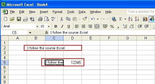
Once that happens, long texts are not fully displayed, but the information in the cell is retained.
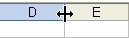
We can see the text by adjusting the column width, by clicking and dragging on the line between two columns.
More of this in another lesson.
Insert numbers in cells
In “Excel”, numbers consist only of numbers, they may not have letters, otherwise it is not considered as a number, but as a text.
And to my knowledge, we can still have text but with no calculations.
So we use only numbers (positive or negative) and we may use a comma.
When a number exceeds the width of a column, this will be represented as:
1. “Pounds notation”: # # # # # #
or as
2. ‘Scientific notation”: 1.34 E 10.
In both cases, we cannot get much from looking at it, so, we increase the width of the column.
Although notation in the pounds will succeed but, we must first change the format of the cell to the scientific notation.
To use the “Scientific notation” , we click”Comma” button  , so that the numbers are legible and the column width adjusts automatically.
“AutoComplete” (“AutoComplete”)
Since ’95 we have the handy feature “AutoFill” in Excel that helps us with recurring data to be prompted automatically.
for example.: we type the word printer in cell A1 and click “Enter”.
When we now start to type in cell A2 with p, Excel will prompt the rest of the word printer as a supplement.
If we do not wish to enter the same word, we just continue typing.
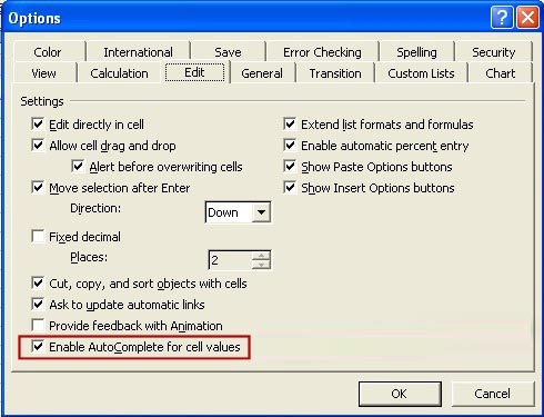
We can disable this feature in the cell.
Click on the “Tools” menu (“Tools”) and choose “Options” (“Options”). In the “Edit” (“Edit”) tab, we click on the checkbox “Enable AutoComplete for cell values” (“Enable AutoComplete for cell values”).So that the tick disappears.
Make your own list
If we need the same lists regularly, we can create custom lists in “Excel” itself, so it is useful to automatically fill in than setting them again and again :
Type your first list in “Excel”.
Then click on “Tools” (“Tools”) and select “Options” (“Options”)
In the “Options” window, we choose the “Custom List” tab (“Custom List”)
Click on “Range” (“Range”)
Select all cells for the “Range” on the “Worksheet” and press “Enter “.
Click below on the “Import” (“Import”) option.
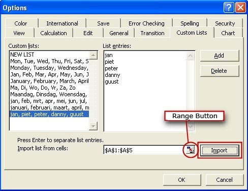 And click Ok.
Now you can also list it in all “Worksheets” in all workbooks in “Excel” to automatically fill data. This can be done by typing the first item and dragging the fill handle down or the right.

Note that, there are standard frames available in “Excel” in the left half of the dialog.
More on this in Lesson 3 – “Auto Fill”.
“Zoom In / Out” of the “Worksheet”
We can resize our “Worksheet”.
We use the “Zoom” button 
We can set the zoom proportion by choosing from the list or manually typing in it.
First select the fields you want to zoom in or zoom out, and then click the “Selection” choice (“Selection”) in the dropdown menu of the “Zoom” button .
Editing multiple “Workbooks “
There will be times when we want to copy data from one “Workbook” to another “Workbook.”
We open both “Workbooks” in Excel, select and copy the data from our source “Workbook”.
To navigate between our different workbooks we click on Window (Window) in the menu bar. In the drop-down menu that opens, we find all open workbooks again.
The one with the checkmark in front is where you are currently working.
We click on the “Copy” button 
Then we open our second “Worksheet” and select the cell where we want to insert the data.
Then we click on the “Paste” button 
Rename “Workbooks”
Once you’ve saved the file, you can still change its name later.
You can also download files that you have changed or in which nothing was done saved under a different name, or at another location.
Simply select the “File” menu bar (“File”) – “Save as ..”. (“Save as ..”)


