Sharing: “Workbooks” (“Share Workbook”)
We can “Share workbook” with other users on a network, and make simultaneous changes.
There are a few things to keep in mind when we do “Share workbook”. The following operations can not be changed or added:
- “Merge cells”
- “Conditional formatting”
- “Data validation”
- “Charts”
- “Images”
- “Objects” (including “Drawing objects”)
- “Hyperlinks”
- “Scenarios”
- “Statements”
- subtotals
- “Data Tables”
- ” PivotTable reports”
- “Workbook” and “Worksheet protection”
- “Macros”
Therefore, do these things before you share the “Workbook”.
To share a “Workbook” we first open our “Workbook”.
Then we select “Tools” – “Share Workbook” from the menu bar.
This opens the dialog “Share Workbook”:
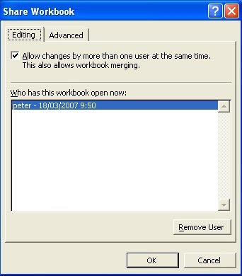
Select the “Editing” tab and check the box “Allow changes by more than one user at the same time”
Then choose the “Advanced” tab to set additional options.
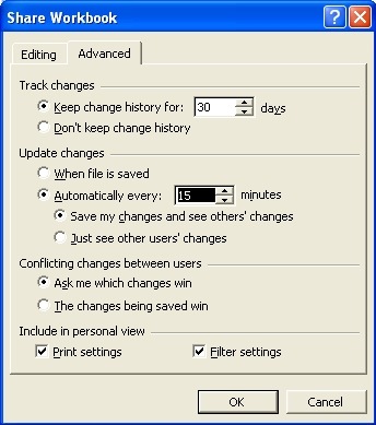
In the upper section of the “Advanced” tab, we can set how long we can track the changes.
In the second section, we set when we want to save changes.
In the third section we propose in what happens when changes made by different users come into conflict with each other.
And in the last section we can use “Print” and “Filter Settings” to personalize the display or view.
Click OK if you are satisfied with the options you set, and click ‘OK’ when asked if you want to save changes.
Once this is done, other users can make changes.
When two users make changes in the same cell, Excel will display a dialog “Resolve Conflicts”.
In this dialog, we see the details of any change which gives rise to a conflict.
To retain your changes, click “Accept Mine” and to retain changes made by others, select “Accept Others”
You can also choose “Accept All Mine” or “Accept All Others”, as per requirement.
Surely this will only happen when we “Ask me which changes win” have checked in the dialog box “Share Workbook” on the “Advanced” tab.
When we no longer want to “Share Workbook” with others, we choose “Tools” from the menu bar, select “Share Workbook” and in the dialog we click again on “Allow changes by more than one user at the same time”.
And click OK.
“Highlight Changes”
To highlight changes we click on “Tools” in the menu bar: select “Track Changes” and click “Highlight Changes”
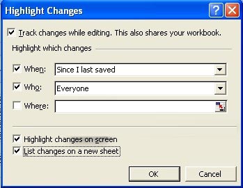
In the dialog that appears, we can select the following options:
“Track Changes while Editing”: This should always be checked if we want to detect changes.
“When”: Here we have several options from which we must make a choice. It does not need a lot of explanation.
“Who”: Here we return a list, which seems clear to me.
“Where”: Here we can enter the “Range” we want to change control for.
In the second section of the dialog we can choose to highlight changes we have made on our screen, and / or on a “New worksheet “.
Click Ok.
Accept Changes
After seeing the changes we can choose to accept it or not.
To do this we click on “Tools” from the menu bar, select “Track Changes” and choose “Accept or Reject Changes”.
In the dialog that opens, we filter the changes by clicking the boxes “When”, “Who”, and “Where”, in order to limit our list.
Once all your selections are completed, click OK.
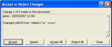
In the window that appears, we see what has changed, by “Whom” and “When”.
Click “Accept” or “Accept All” to accept them, click “Reject” or “Reject All” to refuse.
When multiple changes have happened to a cell, we must first select what we want to preserve.
The “Reviewing toolbar” (“Reviewing Toolbar”)
We use the “Reviewing toolbar” to give comments in cells or to view changes in a shared folder.

A brief explanation of the different buttons:
| “New comment” | “Delete comment “ | |||
| “Edit comment” | hide comments written | |||
| “Previous” comment | remove written comments | |||
| “Next” remark | create outlook task | |||
| hide comment | update file | |||
| hide all comments | send to mail recipient | |||
| reply with changes | ||||
| end review | ||||
“Insert Comment”
When we enter formulas, or make changes in a cell, it may be useful to give some comments about this so others who work with this worksheet find it easy to read.
For example, we would have to add a comment to a cell whose “Function” or “Formula” needs to be explained.
More than once, we want to give comments on changes we have made in a cell, which can explain their usefulness to us and other users.
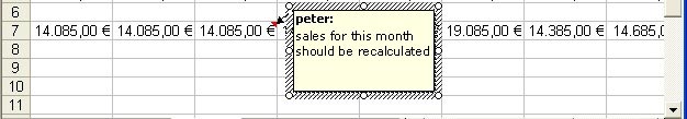
Cell comments are small text frames that are assigned to a cell.
When someone moves his mouse pointer over the cell, there will be a popup window with our comment.
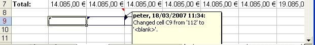
Cells in which a comment was made, have a small red triangle in the upper right corner.
We can easily add a comment to a cell by clicking “New Comment”![]() button.
button.
Or by right-clicking the cell and choosing from the popup menu “Insert Comment”.
The comment text is displayed along with the name of the person making the comment.
When we are ready to give our remark, we click somewhere on our worksheet.
Our cell now appears with the red triangle.
Managing comments
We change our comment by clicking the “Edit Comment” ![]() button.
button.
This button is visible only if our cell already has a comment.
We right click the cell and choose “Edit Comment” from the popup menu.
To delete a comment, we select the cell and click the “Delete Comment” ![]() button.
button.
We right click the cell and choose “Delete Comment” from the popup menu.
View comments
Moving the mouse pointer over the cell, we can view the comment.
But if we have multiple observations in different cells, it may be helpful to read these comments one by one.
We can do this by clicking the “Previous”![]() and “Next”
and “Next” ![]() .
.
By clicking the “Show all Comments” button![]() , we see all the comments in our “Worksheet” and by clicking it once again, hide all comments .
, we see all the comments in our “Worksheet” and by clicking it once again, hide all comments .
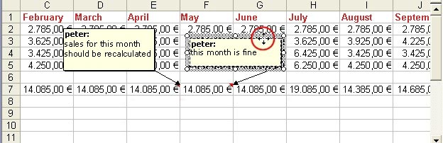
When comments are overlapping, we can shift by moving the mouse pointer over the edge of the comment which has to move, to change it in a cross with arrows, and then click and drag left, right, up or down.
Printing Comments
We have the choice to print our comments at the end of our “Worksheet” or in the “Worksheet”.
Choose “File” in the menu bar and select “Page Setup”.
In the “Print” section, “Comments” box, we can choose between “None” (Don’t print), “At end of sheet” (at the end of the “Worksheet”), or “As Displayed on sheet” (as shown on the “Worksheet”).
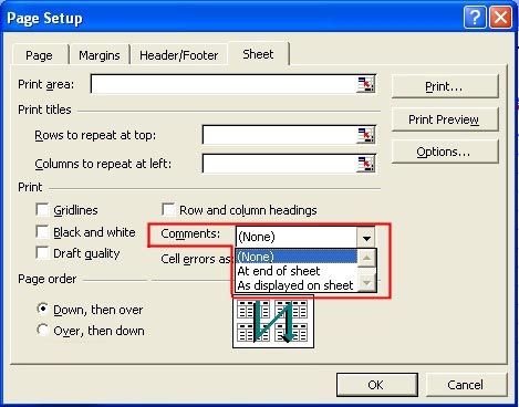
Click on OK when you are satisfied.
Send Spreadsheets
When we have a shared “Workbook”, or a copy thereof, and we want to mail this with Outlook to an employee, we first open our “Workbook”.
Then we select “File” from the menu bar | “Send To” | “Mail Recipient (for Review) …”.
This worksheet will be sent to the receiver so that it can be edited and / or accessed.
And mail it to us after the changes.
When we choose “Mail Recipient (as Attachment) …” will be sent a copy of the “Worksheet”, attached to the e-mail and it will not be used for sharing “Workbooks”.
However, when we have chosen “Mail Recipient (for Review)![]() after having made the changes, the review toolbar automatically opens a way for the reviewer to send the copy back to the sender through mail.
after having made the changes, the review toolbar automatically opens a way for the reviewer to send the copy back to the sender through mail.
When the sender after receiving the modified worksheet opens it again, he will be asked whether he accepts changes or not.
When all changes are made from all employees, click the “End Review” button![]() .
.
“Compare and Merge Workbooks”
When we have copies from different employees with different modifications, we may want to incorporate all those “Workbooks” into one “Workbook”.
There are some requirements that these files should have, before we can do that.
- All “Workbooks” have copies of the original.
- They must all have different names, but in the same directory.
- They may not have “Password”.
- They must all be set to “Track Changes” since their “History” (“History”) should be known.
Also note, when multiple copies are together, the changes made in the last “Workbook” will be replaced when you merge any conflicts in the “Workbook”.
To merge “Workbooks”, we will first verify that these are all located in the same folder.
Then we open our “Workbook” where we want to merge.
We click on “Tools” in the menu bar and select “Compare and Merge Workbooks …”
We save the “Workbook” as seen above.
This opens the dialog “Select Files to Merge into Current Workbook”.
Here we select the different copies of the “Workbooks” that we want to merge.
And click OK.


