Formulas used in data validation.
In Excel 2007 course lessons 066, 067 and 068 and Excel 2010 lessons 70, 71 and 72 , we discussed several options for data validation. In this tip, we will discuss a few more options.
Value of the cell must be higher than parent cell.
As a first example we take a file (1) where we record our weekly (2) gas consumption. To avoid that we enter an incorrect meter reading. Meter readings should be in ascending order, so we use a formula.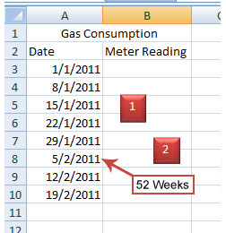
Fill in the initial meter reading in cell B3, click in cell B4, press the Shift key, click in cell B55.
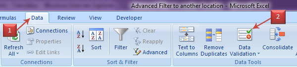
Goto the “Data” on the ribbon and click on “Data Validation”.
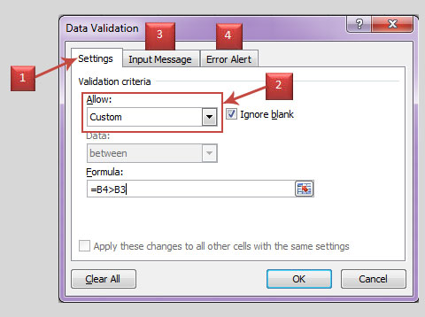
In the ‘Settings’ tab (1) of the “Data Validation” window, choose “Custom” in the “Allow” box (2), in the “Formula” box, type the equal sign “=”, click in the cell B4, type the comparison operator “>” (greater than) and click in the cell B3 (the formula is =B4>B3) and we fill in the appropriate messages in the “Input Message” tab (3) and “Error Alert” tab and click ok.
The data validation is automatically adjusted for the remaining selected cells, we can test this by selecting any cell in which we have applied validation in the window “Data Validation” eg cell B20 and we can see the modified formula for the cell B20, that is = B20> B19.
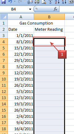
The formula that we enter in the “data validation” must be formulated for the first selected cell, the first selected cell in a selected area is in the lighter color (1).
In the following examples we assume that we selected the cells A1 to A10, and the cell A1 is the first selected cell, and we go to “Data” tab on the ribbon and click on “Data Validation”, select the “Settings” tab of the “Data Validation” window and select “Custom” in the “Allow” box.
No duplicates allowed.
We use the COUNTIF function.
The function counts the number of cells in a range (parameter 1) that meets a criterion (parameter 2) that you specify.
Formula is = COUNTIF ($ A $ 1: $ A $ 10, A1) = 1 and press OK. We make the cells A1: A10 as the absolute parameter range so that it is not adjusted for the cells A2 to A10.
Now we can enter any value only once in the cells A1 to A10.
No weekend days allowed.
If we want to enter the dates of working weekdays (not Sat and Sundays).
We use the functions AND and WEEKDAY.
The AND function is often used expand to combine other functions that perform logical tests.
The WEEKDAY function returns the day of the week for a date. The day is displayed by default as an integer from 1 (Sunday) to 7 (Saturday).
Formula is = AND (WEEKDAY (A1)<>1; WEEKDAY (A1)<>7) and press OK.
Limit total amount
If a certain amount must not be exceeded eg 1000.
Formula is = SUM ($ A $ 1: $ A $ 10)<=1000 and press OK. . We make the cells A1: A10 as the absolute parameter range so that it is not adjusted for the cells A2 to A10.
Now, the total amount for the cells A1 through A10 has a limit of 1000.
Allow only Text
If you are allowed to enter text only.
We use the function: ISTEXT
The ISTEXT verifies that the contents of the cell is text.
Formula is = ISTEXT (A1) and press OK.
Initial
If the text must begin with a certain letter eg X (Note that this is not case sensitive, so both lowercase and uppercase letters are allowed).
We use the function: LEFT
The LEFT function gives the first character or the first number of characters in a string, based on the number of characters we specify. The LEFT function has 2 parameters, namely the text, that is the string with the characters that you want to retrieve and the number of characters, which is optional. The number of characters you want LEFT to retrieve must be greater than or equal to zero.
If the number of characters is greater than the length of the text, then LEFT will return all of the text as a result.
If number of characters parameter is omitted, it assumes the value of 1.
eg. = LEFT (A1) returns the first character in cell A1.
Formula is = LEFT (A1) = “X” and press OK.
Begin letters + text length
If the text must begin with certain letters eg. XYZ, followed by a hyphen, and must exactly be 9 characters long.
We use the function: COUNTIF
Formula is = COUNTIF (A1, “XYZ-?????”) = 1 and press OK. (Note, this is not case sensitive, so both lowercase and uppercase letters are allowed, eg XYZ-ABCDE, xyz-abcde, and in place of the question marks, both letters and numbers allowed therefore XYZ-12ABC is also accepted).
Rating and case combination
If the cell contents should be a combination of numbers and capital letters and a hyphen
eg XYZ-123-ABC.
We use the functions AND, EXACT, UPPER, LEFT, MID, RIGHT, VALUE and LEN.
The EXACT function compares two strings and returns TRUE if the strings are identical and FALSE if it is not the case. A distinction is made between uppercase and lowercase letters. Formatting differences, however, are ignored. Use EXACT to check text entered in a document, this function has 2 parameters, namely text1 is required. The first character string.
text2 is required. The second string.
The function UPPER converts text to uppercase and has 1 parameter, namely the text, which is required. The text you want to convert to uppercase. The text can be a string or a reference.
The function LEFT: see the earlier example
The function MID returns a specific number of characters from a string, starting from the specified position and based on the number of characters specified and consists of 3 parameters, namely text is required. The string with the characters that you want to retrieve.
start_num is required. The position of the first character you want to retrieve. The first character in the text has a value of 1.
number of characters is required. The number of characters you want to retrieve from text to MID.
eg. = MID (A1, 4, 2) returns 2 characters from the 4th character of the contents of cell A1, that is characters 4 and 5 of cell A1.
The RIGHT function displays the last character or the last characters in a string, based on the number of characters you enter and has 2 parameters, namely text is required. The string with the characters that you want to retrieve.
num_chars is optional. The number of characters you want RIGHT to retrieve.
eg. = RIGHT (A1, 3) returns the last 3 characters from cell A1.
The NUMBER function converts a string that represents a number to a number and has 1 parameter namely text is required. The text enclosed in quotation marks or reference to the cell containing the text that you want to convert.
The LENGTH function returns the number of characters in a string.
To put together a long formula, it is easier to first put it in a cell, we can then use the formula aid (1). We do not have the formula aid available in the “Data Validation” window. We take cell B1 for example.
Because there are several conditions that must be met, we begin with the AND function.
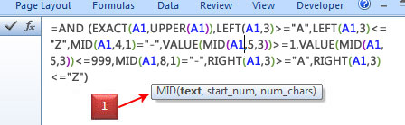
We type =AND ( Then we take the function EXACT that compares 2 values, parameter 1 is cell A1 and parameter 2 is UPPER (A1). We type the closing parenthesis of the function EXACT.
Until now, we have the formula = AND (EXACT (A1, UPPER (A1)).
Any condition for the AND function is separated by commas, so we type the comma ‘,’. The next condition is that the first 3 characters must be greater than or equal to A. Here we use the function LEFT (A1, 3)> = ‘A’, type a comma “,” again. For the next condition, that is the first 3 character have to be smaller than or equal to Z, we use LEFT (A1, 3)<=”Z”
Now we have the formula = AND (EXACT (A1, UPPER (A1)), LEFT (A1, 3)> = ‘A’, LEFT (A1, 3)<=”Z”.
We again type a comma to enter the next condition. Here we must ensure that the fourth character must be a hyphen, so we use the function MID, MID (A1, 4, 1) = “-”
Now we have the formula = AND (EXACT (A1, UPPER (A1)), LEFT (A1, 3)> = “A”, LEFT (A1, 3)<=”Z”, MID (A1, 4, 1) = “-“. We again type a comma as a separator for the next condition.
Now we want to ensure that three digits from the fifth character must be greater than or equal to 1, we use the VALUE and MID functions, VALUE (MID (A1, 5, 3))> = 1, type a comma again for the next condition, three digits from the fifth character should be smaller or equal to than 999 VALUE (MID (A1, 5, 3)) <= 999.
Now we have the formula = AND (EXACT (A1, UPPER (A1)), LEFT (A1, 3)> = “A”, LEFT (A1, 3)<=”Z”, MID (A1, 4, 1) = “-“, VALUE (MID (A1, 5, 3))> = 1, VALUE (MID (A1, 5, 3))<=999.
We type a comma for the next condition. The eighth character must be a hyphen, MID (A1, 8, 1) = “-“.
Now we have the formula = AND (EXACT (A1, UPPER (A1)), LEFT (A1, 3)> = “A”, LEFT (A1, 3)<=”Z”, MID (A1, 4, 1) = “-“, VALUE (MID (A1, 5, 3))> = 1, VALUE (MID (A1, 5, 3)) <= 999, MID (A1, 8, 1) = “-“.
We type a comma for the next condition.
The last three characters, three characters are greater than or equal to A, we use the RIGHT functionRIGHT (A1, 3)> = ‘A’, type a cooma for the next condition, that is, the last 3 characters must be less than or equal to Z, RIGHT (A1, 3)<=”Z”
The formula is now = AND (EXACT (A1, UPPER (A1)), LEFT (A1, 3)> = “A”, LEFT (A1, 3)<=”Z”,MID(A1,4,1)=”-“,
VALUE (MID (A1, 5, 3))> = 1, VALUE (MID (A1, 5, 3)) <= 999, MID (A1, 8, 1) = “-“,
RIGHT (A1, 3)> = “A”, RIGHT (A1, 3) <= “Z”
We again type a comma “,” and to determine the length we take the LEN function, we type LEN (A1) = 11 and we type the closing parenthesis ‘)’ of the AND function and enter Ctrl + Enter so that the cell containing the formula is selected.
The formula typed is:
AND (
EXACT (A1, UPPER (A1)),
LEFT (A1, 3)> = “A”,
LEFT (A1, 3) <= “Z”,
MID (A1, 4, 1) = “-“,
VALUE (MID (A1, 5, 3))> = 1,
VALUE (MID (A1, 5, 3)) <= 999,
MID (A1, 8, 1) = “-“,
RIGHT (A1, 3)> = “A”,
RIGHT (A1, 3) <= “Z”,
LEN (A1) = 11)
To know if the formula is working properly, in cell A1, we type the correct letter and number combination that should give the result “TRUE”, and a bad combination to give us the result “FALSE”.
We first delete the contents of cell A1. If we do not do this and there is a bad combination in the cell, then this error is not recognized as wrong combination after entering the formula in the “Data validation” window. Then select it and copy the formula from cell B1 from the formula bar, select some cells eg A1 to A10, go to the “Data” tab on the ribbon and click on “Data Validation”. On the “Settings” tab of the “Data Validation” window, choose “Custom” in the “Allow” box, and paste the formula in the space provided for “Formula” and click OK.
So you see, with the option “Custom” for data validation, the possibilities are virtually unlimited.


